Supervised Learning algorithms with R (part 1)

As I mentioned in an earlier post, machine learning algorithms are categorized into three main types :

• Supervised learning algorithms
• Unsupervised learning algorithms
• Reinfocement learning algorithms

In this article, we will only talk about some of machine learning supervised algorithms. We’ll also see examples using R programming language.

First of all, I would like to remind you that supervised learning is a machine learning algorithm that tries to find a function mapping an input to a given output based on a set of examples. Basically, each of these examples (called training set) consists of the input $X$ and the desired output $Y$. In other words, we try to approximate the function $f$ such that $f(X)=Y$ using previously labelled data as learning examples. The performance of such a model is evaluated upon its ability to generalize onto new data that is unlabeled.

K-Nearest Neighbours

K-Nearest Neighbours (KNN) is a simple Machine Learning algorithm based on Supervised Learning technique. It can be used for both regression and classification, but it is mostly used in classification.

Suppose we have two categories : Category $A$ and Category $B$, and we have a new data point $x$ that we want to know to which category it belongs.

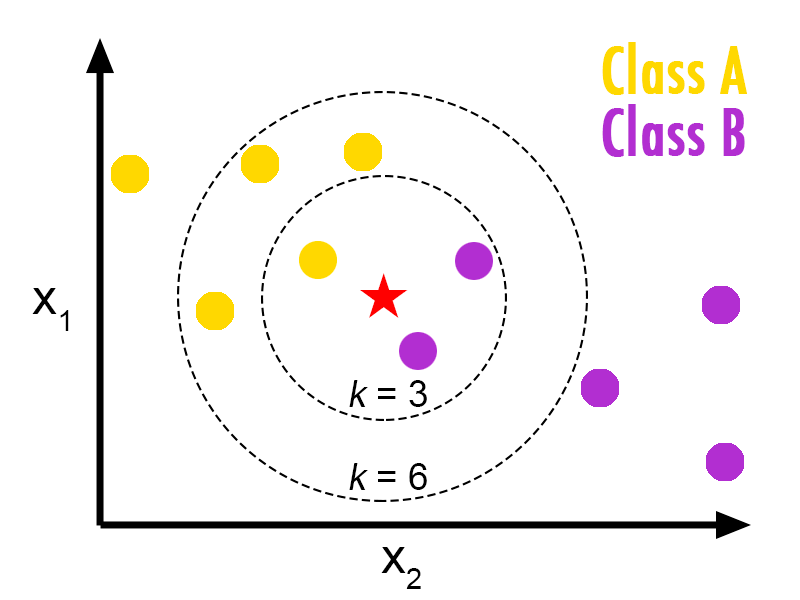
KNN algorithm is comprised of the following steps :

• Step 1 : Select K, number of neighbours
• Step 2 : Calculate the distance of between $x$ and each of the other data points (we can use the Euclidian distance or others)
• Step 3 : Take the K nearest neighbors as per the calculated Euclidean distance.
• Step 4 : Among these k neighbors, count the number of the data points in each category.
• Step 5 : Assign the new data points to that category for which the number of the neighbor is maximum.

NB 1 : The Euclidian distance between two points $a_1(x_1,y_1)$ and $a_2(x_2,y_2)$ is calculated as follows : $$d(a_1,a_2)=\sqrt{(x_1-x_2)^2+(y_1-y_2)^2}$$

NB 2 : As can be seen, there are no parameters that need to be learned during training to determine whether a new observation belongs to class 𝐴 or 𝐵. The only parameter used in K-Nearest Neighbours is K, which is a predetermined value. The algorithm simply works by looking at the training samples, calculating distances and finding the K examples in the training set that are closest to the new observation. Thus, KNN is a non-parametric, supervised (needs training labels) learning algorithm.

NB 3 : KNN does support categorical variables as features, simply because we cannot calculated the distance from them.

The hands-on example¹ that we will work on will use the Sonar data set (signals) from mlbench library. Sonar is a system for the detection of objects under water and for measuring the water’s depth by emitting and detecting sound pulses (the complete description can be found →here). For our purposes, this is a two-class (class $R$ and class $M$) classification task with numeric data.

First of all, let’s install the required libraries :

# install the packages (note: this may take some time)
install.packages("class")
install.packages("caret")
install.packages("mlbench")
install.packages("e1071")

library(class)
library(caret)
require(mlbench)
library(e1071)
library(base)
require(base)

Step 1 : Loading the data

Let’s load the Sonar dataset and look at the first five rows :

data(Sonar)
head(Sonar)

Step 2 : Preparing and exploring the data

nrow(Sonar)
ncol(Sonar)

This will display the number of lines (208 observations) and the number of columns (61 variables), all numerical except for the Class variable which is categorical.

Let’s check how many $R$ classes and $M$ classes Sonar contains :

base::table(Sonar$Class)

Now let’s see if it contains any NA values in its columns :

apply(Sonar, 2, function(x) sum(is.na(x))) 

We are going to manually split Sonar into training and test sets. Here, we will dedicate 70% of the dataset for traing, and the rest for testing :

SEED <- 123
set.seed(SEED)
data <- Sonar[base::sample(nrow(Sonar)), ] # shuffle data first
bound <- floor(0.7 * nrow(data))
df_train <- data[1:bound, ] 
df_test <- data[(bound + 1):nrow(data), ]
cat("Number of training and test samples are ", nrow(df_train), nrow(df_test))

Now, let’s create the following dataframes :

X_train <- subset(df_train, select=-Class)
y_train <- df_train$Class
X_test <- subset(df_test, select=-Class) # exclude Class for prediction
y_test <- df_test$Class

tep 3 : Training a model on data

Now, we are going to use knn function from class library with $K=3$ :

knn_model <- knn(train=X_train,
                 test=X_test,
                 cl=y_train,  # class labels
                 k=3)
knn_model

If you run the code above, you’ll see the prediction made by knn_model with $K=3$ on X_test.

Step 4 : Evaluate the model performance

In order to see how many classes have been correctly or incorrectly classified, we can create a confusion matrix as follows :

conf_mat <- base::table(y_test, knn_model)
conf_mat

To compute the accuracy, we sum up all the correctly classified observations (located in diagonal) and divide it by the total number of classes :

cat("Accuracy: ", sum(diag(conf_mat))/sum(conf_mat))

To assess whether $K=3$ is a good choice and see whether $K=3$ leads to overfitting/underfitting the data, we could use knn.cv which does the leave-one-out cross-validations for training set (i.e., it singles out a training sample one at a time and tries to view it as a new example and see what class label it assigns).

knn_loocv <- knn.cv(train=X_train, cl=y_train, k=3)
knn_loocv

Let’s create a confusion matrix to compute the accuracy of the training labels y_train and the cross-validated predictions knn_loocv, same as the above :

conf_mat_cv <- base::table(y_train, knn_loocv)
conf_mat_cv
cat("LOOCV accuracy: ", sum(diag(conf_mat_cv)) / sum(conf_mat_cv))

The difference between the cross-validated accuracy and the test accuracy shows that $K=3$ leads to overfitting. Perhaps we should change $K$ to lessen the overfitting.

Step 5 : Improve the performance of the model

There are a couple things we can do in order to improve the performance of our model :

• Centering and scaling data : these are forms of preprocessing numerical data (not suitable for categorical data). Centering a variable means subtracting the mean of the variable from each data point so that the new variable’s mean is 0. And scaling consists of multiplying each data point by a constant in order to alter the range of the data.
• Performing a cross-vaidation : this consists of dividing the data into a finite number of subsets. Through each iteration, a subset is set aside, and the remaining subsets are used as the training set. The subset that was set aside is used as the test set (prediction). We will use caret library for this purpose.

This is a method of cross-referencing the model built using its own data :

SEED <- 2016
set.seed(SEED)
# create the training data 70% of the overall Sonar data.
in_train <- createDataPartition(Sonar$Class, p=0.7, list=FALSE) # create training indices
ndf_train <- Sonar[in_train, ]
ndf_test <- Sonar[-in_train, ]

Here, we specify the cross-validation method we want to use to find the best $K$ in grid search.

# lets create a function setup to do 5-fold cross-validation with 2 repeat.
ctrl <- trainControl(method="repeatedcv", number=5, repeats=2)

nn_grid <- expand.grid(k=c(1,3,5,7))
nn_grid

set.seed(SEED)

best_knn <- train(Class~., data=ndf_train,
                  method="knn",
                  trControl=ctrl, 
                  preProcess = c("center", "scale"),  # standardize
                  tuneGrid=nn_grid)
best_knn

Running the code above, you’ll find out that $K=1$ has the highest accuracy from repeated cross-validation.

Decision Trees

Decision Trees are one of the most powerful predictive classification models. They are based on the analysis of a set of data points that describe the type of object we want to classify. A Decision tree is a flowchart like tree structure, where each internal node denotes a test on an attribute, each branch represents an outcome of the test, and each leaf node (terminal node) holds a class label.

In our practical example², we’ll try to classify a set of mushrooms as either edible or poisonous based on features like its cap type, color, odor, shape of its stalk, etc.

The algorithm behind Decision trees uses probabilities. For example, if many mushrooms that have large caps are poisonous, the algorithm will assume that the probability of large-cap mushrooms being poisonous is high. When the model is complete, we have a tree-like structure composed of what are called decision nodes, which ask our data point questions about its features, and leaf nodes, which tells us what classification the decision tree thinks our data point is.

The goal of a decision tree is to split the dataset on based on attributes. But how to find the best feature in each node to split?

To answer this question, let’s first define the Entropy.

Entropy is the amount of information disorder, or the amount of randomness in the data. It is calculated for each node and it depends on how much random data that node contains. In decision tree we are looking for a trees that have smallest entropy in their nodes. The entropy is used to calculate the homogeneity of the samples in that node. If the samples are completely homogeneous the entropy is zero and if the sample is an equally divided it has entropy of one. It means, if all data in a node are either poisonous or edible, then the entropy is zero, but if the half of data are poisonous and other half are edible, then the entropuy is one. In our example, we can calculate the Entropy of our target class using the following formula :

$$Entropy = - p(edible)log(p(edible)) - p(poisonous)log(p(poisonous))$$

Decision trees use another metric on which decisions are based : Information gain. We can think of it as the opposite of entropy. The more randomness decreases, the more information we gain, and vice-versa. Thus, while building a decision tree, we choose the attributes with the highest information gain. $$\text{Information Gain = entropy(parent) – [average entropy(children)]}$$

Algorithm :

  1. Calculate entropy of the target field (the class label) for whole dataset.
  2. For each attribute:
    - split the dataset on the attribute
    - calculate entropy of the target field on splited dataset, using the attribute values
    - calculate the information gain of the attribute
  3. select the attribute that has the largest informmation gain
  4. Branch the tree using the selected attribute
  5. stop, if it is a node with entropy of 0, otherwise jump to step2

Decision tree with R

We will start by loading the data. We’ll use UCI’s Mushroom dataset. Since this dataset is not inbuilt into R, we need to download it and load it into R :

download.file("https://ibm.box.com/shared/static/dpdh09s70abyiwxguehqvcq3dn0m7wve.data", "mushroom.data")

After downloading the file, we need to create a data frame to house the observations in the dataset. Since the dataset is structured using comma-separated values, we can use the read.csv function :

mushrooms <- read.csv("mushroom.data", header = F)
mushrooms

Once that’s done, we have the data loaded up. However, the way that it is structured isn’t the most intuitive. In the code cell below, we are adding the column names to the data frame with the colnames function. Additionally, since our data frame is composed of factors, we can rename some of these factors to something more easily understood by us using levels.

# Define column names for the mushrooms data frame.
colnames(mushrooms) <- c("Class","cap.shape","cap.surface","cap.color","bruises","odor","gill.attachment","gill.spacing",
                         "gill.size","gill.color","stalk.shape","stalk.root","stalk.surface.above.ring",
                         "stalk.surface.below.ring","stalk.color.above.ring","stalk.color.below.ring","veil.type","veil.color",
                         "ring.number","ring.type","print","population","habitat")
head(mushrooms)

# Define the factor names for "Class"
levels(mushrooms$Class) <- c("Edible","Poisonous")

# Define the factor names for "odor"
levels(mushrooms$odor) <- c("Almonds","Anise","Creosote","Fishy","Foul","Musty","None","Pungent","Spicy")
# Define the factor names for "print"
levels(mushrooms$print) <- c("Black","Brown","Buff","Chocolate","Green","Orange","Purple","White","Yellow")
head(mushrooms)

Now let’s build our model. We are going to use rpart library to create the decision tree, and rpart.plot to visualize it. But first, install rpart.plot if it’s not already installed.

install.packages("rpart")
install.packages("rpart.plot")

# Import our required libraries
library(rpart)
library(rpart.plot)

To create our decision tree model, we can use the rpart function. rpart is simple to use: you provide it a formula, show it the dataset it is supposed to use and choose a method (either “class” for classification or “anova” for regression).

A great trick to know when handling very large structured datasets (our dataset has over 20 columns we want to use!) is that in formula declarations, one can use the . operator as a quick way of designating “all other columns” to R. You can also print the Decision Tree model to retrieve a summary describing it.

# Create a classification decision tree using "Class" as the variable we want to predict and everything else as its predictors.
myDecisionTree <- rpart(Class ~ ., data = mushrooms, method = "class")
# Print out a summary of our created model.
print(myDecisionTree)

Now that we have our model, we can draw it to gain a better understanding of how it is classifying the data points. We can use the rpart.plotfunction – a specialized function for plotting trees – to render our model. This function takes on some parameters for visualizing the tree in different ways – try changing the type (from 1 to 4) parameter to see what happens!

If you run the code above, you’ll see that our decision tree has perfect accuracy when classifying poisonous mushrooms, and almost perfect accuracy when dealing with edible ones.

newCase  <- mushrooms[10,-1]
newCase

predict(myDecisionTree, newCase, type = "class")

Model accuracy :

Let’s split our dataset into traing set and test set :

## 75% of the sample size
n <- nrow(mushrooms)
smp_size <- floor(0.75 * n)

## set the seed to make your partition reproductible
set.seed(123)
train_ind <- base::sample(c(1:n), size = smp_size)

mushrooms_train <- mushrooms[train_ind, ]
mushrooms_test <- mushrooms[-train_ind, ]

newDT <- rpart(Class ~ ., data = mushrooms_train, method = "class")

result <- predict(newDT, mushrooms_test[,-1], type = "class")

head(result)

head(mushrooms_test$Class)

base::table(mushrooms_test$Class, result)

That’s it! See you on another cool article :)