Supervised Learning algorithms with R (part 2)
In a previous article, we have explained the principles of K-Nearest Neighbours and Decision Trees and seen hands-on examples of how these models can be created using R programming language. In this article, we will continue on the same track and see other supervised learning algorithms, namely Linear Regression and Logistic Regression.
Regression is one of the most important fields in statistics and machine learning. Its objective is to find relationships between variables. On use case of regression is when you try to find out how some features of employees – such as experience, role, education and city – influence their salaries. To solve this problem, we apply regression on a dataset comprised of a large enough amount observations, each representing the data (features) related to each employee.
When do we need Regression?
Basically, regression is used to answer the following questions :
- Does X influence Y?
- If the answer is yes, how is Y influenced?
- In other words, how Y is related to each of the input features, and how these features are correlated?
Regression is almost always present in decision-making processes in all fields such as economy, demographic analysis, real estate industry, education, etc.
Linear Regression
Linear Regression is the simplest regression method and the most widely used because of the ease of interpreting results. It is a predictive model used to predict the outcome value of an outcome variable (dependent variable) Y based on one or more input predictor variables (independent variables) X. The aim is to establish a linear relationship (a mathematical formula) between the predictor variable(s) and the response variable, so that we can use this formula to estimate the value of the response Y, when only the predictors values are known.
A linear regression between dependent variable $Y$ and a set of independent variables $X=(x_1,…,x_n)$ assumes that there is a linear relationship between $X$ and $Y$, i.e. : $$Y=\beta_0 + \beta_1x_1 + … + \beta_nx_n + \varepsilon$$ The equation above is called the regression equation. $\beta_0, \beta_1, …, \beta_n$ are called the regression coefficients, and $\varepsilon$ is the random error.
Linear regression calculates the predicted weights $\hat{\beta}_0, \hat{\beta}_1, …, \hat{\beta}_n$ that define the regression function : $$f(X)=\hat{\beta}_0 + \hat{\beta}_1x_1 + … + \hat{\beta}_nx_n$$
The estimated response $f(X^{(i)})$ of each observation $i=1,…,N$ should be as close as possible to the corresponding actual response $Y^{(i)}$. The differences $Y^{(i)}-f(X^{(i)})$ for all the observations $i=1,…,N$ are called residuals. Regression is about determining the best predicted weights, that is the weights corresponding to the smallest residuals.
In order to obtain the best weights, we try to minimize the sum of squared residuals (SSR) for all observations $i=1,…,N$ : $$SSR=\sum_i (Y^{(i)}-f(X^{(i)}))^2$$ This method is called the method of ordinary least squares.

After fitting our model, we would eventually want to measure how good the fit is. One way to do it is by calculating $R^2$ also called Coefficient of determination.
The variation of the actual responses $Y^{(i)}$ is partly due to their dependence on $X$. But there is also a part of the overall variation that is intrinsic to the output itself.
$$R^2=\dfrac{\text{Variance explained by the model}}{\text{Total variance}}=1-\dfrac{SSR}{TSS}$$
$SSR$ : sum of squared residuals
$TSS$ : total sum of squares
$R^2$ is the amount of variation in $Y$ that can be explained by its relationship with $X$. Usually, the larger the $R^2$, the better the regression model fits your observations and can better explain the variation of the output with different inputs. $R^2=1$ corresponds to the case where $SSR=0$ , which is the perfect fit.


Simple linear regression
Simple linear regression is the simplest case of linear regression. It helps us summarize and study relationships between two continuous (quantitative) variables $X=x$ (the input, which is comprised of a single feauture) and $y$ (the output).

In the plot above, the red line represents the regression function $f(x)=b_0+b_1x$. The goal is to estimate the values of $b_0$ (intercept) and $b_1$ (coefficient or slope) that minimize the SSR.
Multiple Linear Regression
Multiple or multivariate linear regression is a case of linear regression with two or more independent variables. For example, if there are just two independent variables, the estimated regression function is $f(x_1,x_2)=b_0+b_1x_1+b_2x_2$

The goal of regression is to determine the values of the weights $b_0$, $b_1$, and $b_2$ such that this plane is as close as possible to the actual responses and yield the minimal SSR.
The case of more than two independent variables is similar, but more general. The estimated regression function is $f(x_1,…,x_r)$, and there are $r+1$ weights to be determined when the number of inputs is $r$.
Polynomial Regression
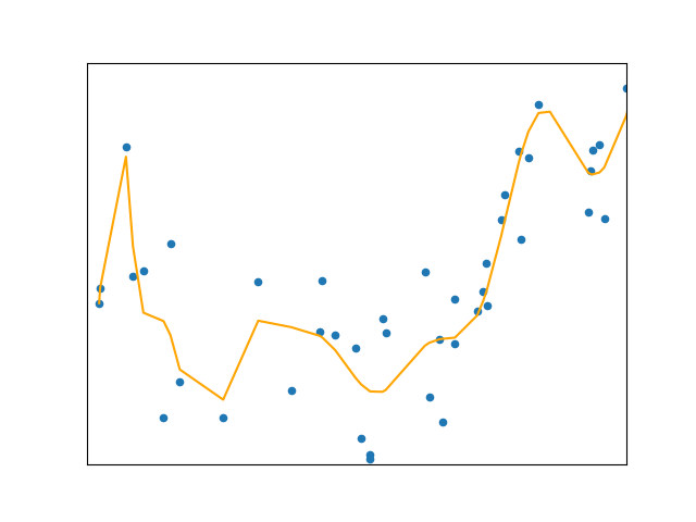
Linear Regression assumes a linear relationship between variables. But in most real life cases, data is too complex to be modeled linearly. In order to overcome under-fitting, we need to increase the complexity of the model. So when it comes to generating a curve that best captures the data (as in the figure below), Polynomial Regression may be the answer.
Polynomial regression can be regarded as a generalization of linear regression in which we assume the polynomial dependence between the output and inputs and, consequently, the polynomial estimated regression function. In other words, in addition to linear terms like $b_1x_1$, regression function also includes non-linear terms such as $b_2x_1^2$, $b_3x_1^3$, or even $b_4x_1x_2$, $b_5x_1^2x_2$ and so on.
Note that a polynomial regression problem can be solved by transforming it into a linear model, which is easier to solve. For example, if we consider this following polynomial regression function $f(x)=b_0+b_1x+b_2x^2$, the term $x_2$ can be considered as a new feature. The previous regression function is then equivalent to the following multilinear regression function $f(x_1,x_2)=b_0+b_1x_1+b_2x_2$.
Similarly, in the case of a polynomial regression problem with multiple input variables, each non-linear term in the regression function can be considered as a new input ($x_1^2$, $x_1x_2$, $x_2^2$, …). What you get as the result of regression are the values of the weights ($b_0,b_1,b_2…$) which minimize SSR.
Implementing Simple Linear Regression with R
Let’s see a concrete example on how to implement simple linear regression in R programming language. We will use